Timing in R: Best Practices for Accurate Measurements

Timing in R is a requirement for data analysis for R developers. It is required for optimizing your R code. In this tutorial we will cover all your options and describe pros and cons of each.

Without knowing your options can be the difference between a success and failure if your code doesn’t perform well.

Code execution time affects the speed of the analysis and the overall efficiency of the process. Therefore, mastering timing techniques in R is crucial for any data analyst, scientist, or R programmer.

As you already suspect, R provides various tools and functions to help users measure and optimize the timing of their code. These tools can help programmers identify bottlenecks in their R code and ultimately improve performance, hopefully. This post will explore our options.

R offers several packages for timing analysis, such as tictoc, and also for benchmark comparisons, such as microbenchmark and rbenchmark. We’ll cover both of these and more in the examples below.

Noteworthy is timing is not only about performance optimization. Timing R can also play a significant role in reproducibility and accuracy; in other words, consistency.

Because the timing of R code execution affects the randomness and variability of the results, it can lead to inconsistent or unreliable findings. So, it can be critical to understand the timing implications of different functions and algorithms and how they affect the outcome of the R program. I’ll call out warnings of this in the examples below.

Let’s continue now with our exploration of options and best practices for timing in R code.

Understanding Timing in R

What is Timing in R?

Timing in R is the amount of time it takes for a particular operation, function, or set of operations to execute in R code. Knowing how and why to measure R timing is usually a sign of moving from beginner to more advanced R programer. Because first you should focus on getting your code to work, followed by optimizing your R code execute faster.

Why is Timing Important in R?

Timing is important in R because it can help identify slow, inefficient areas of R code. By measuring the time it takes for portions of your program to execute, it can help you identify bottlenecks which provides opportunities to optimize and improve performance.

R timing can be useful for comparing the performance of algorithms or how you have approached initial versions of implementation. Comparing versions can help choose the best approach and ensure code is running efficiently.

Overall, understanding timing in R is an important skill for any R developer.

Measuring Timing in R

As mentioned, R timing is an essential in R development. In R, timing can be measured using various functions and techniques. This section explores the different options of measuring timing in R through examples.

R Timing Examples Setup

In the following sections, we will run through some examples of how to time your R code. These R timing examples will utilize sample datasets provided by the “palmerpenguins” library and conveniences “tidyverse” library. (Links to both libraries in Resources below)

Here’s the R code to setup the upcoming R timing examples

# setting seed to make results reproducible
set.seed(1234)

# Loading libraries needed
library(tidyverse)
library(palmerpenguins)

# Inspecting data
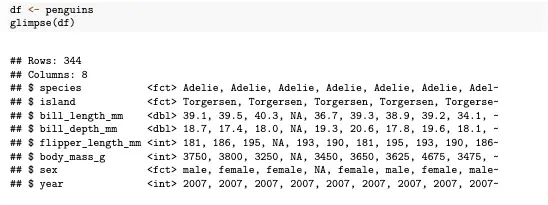
df <- penguins
glimpse(df)

# saving to directory
write.csv(df, 'data.csv')
saveRDS(df, 'dataset.rds')

If you run this code above, you’ll see various outputs such as the following from glimpse available from the tidyverse library:

Timing in R code example data set output

Timing Functions in R

Let’s start our exploration of timing in R options with some built-in functions. R provides several built-in functions for measuring timing, including Sys.time(), system.time(), and proc.time().

As we will see below, Sys.time() is used to determine current system time and can called multiple times to calculate elapsed time.

The system.time() function we will explore below returns the amount of CPU time used by the R process.

The proc.time() function returns the amount of CPU time used. It can useful for measuring the time taken by a sequence of expressions or function calls.

Let’s take a look at examples of each of these now.

R Timing with system.time

# Measuring duration to load file to our workspace with system.time()

# csv file
system.time(read.csv('data.csv'))

# rds file
system.time(readRDS('dataset.rds'))

Example output of these two system.time functions:

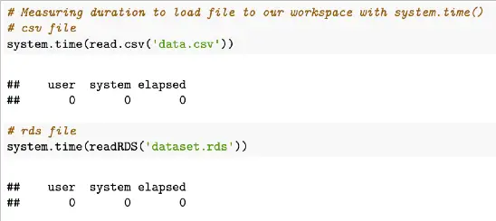
system.time() outputs include an object with “user” which represents the user CPU time in seconds, “system” which represents the system CPU time in seconds, and “elapsed” representing the elapsed time in seconds.

Note: timing results obtained from system.time() may vary depending on various factors such as system load, CPU speed, and the size of the input data, but for this script and others that follow below, we used set.seed() to ensure reproducibility.

R Timing with Sys.time

# Measuring duration to load file to our workspace with Sys.time()

# csv file
start <- Sys.time()
df <- read.csv('data.csv')

Sys.time() - start

# rds file
start_1 <- Sys.time()
dd <- readRDS('dataset.rds')
Sys.time() - start_1

Sample output of Sys.time example above

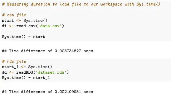
In this example, we can see the time to load a csv file is 0.02907991 seconds and the time for loading an RDS file was 0.0259881 seconds.

The Sys.time() function is used to measure the current system time. As shown in the example above, Sys.time() can be used to mark both the start and end time; i.e. Sys.time() - start

Sys.time() in R gives provides current system time, but again, it may vary slightly due to factors like system load, clock synchronization, and time zone settings.

R Timing with proc.time

# Measuring duration to load file to our workspace with proc.time()

# csv file
start_2 <- proc.time()
df <- read.csv('data.csv')

proc.time() - start_2

#rds file
start_3 <- proc.time()
dd <- readRDS('dataset.rds')

proc.time() - start_3

Example output from these proc.time shown above:

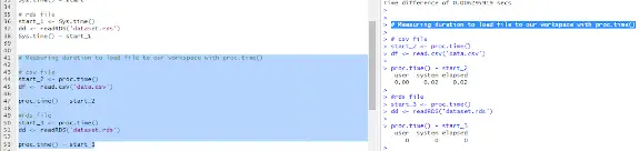
In this example and screenshot of output from RStudio, proc.time() is used to record the start time before and after calling the read.csv() and readRDS() functions similar to the previous Sys.time examples.

The result processing time contains information about user CPU time, system CPU time, and elapsed time in seconds. We can use this result to assess the performance of both functions.
Again, because it’s similar to previous examples, it’s important to note proc.time() measures CPU time, which represents overall time spent executing code and may not capture CPU time spent waiting for I/O operations or other external factors.

R Built-In Functions Timing Differences and Recommendation

You are probably wondering the differences in the three examples above.

system.time() measures CPU time used by a specific expression or function
Sys.time() gives the current system time for time-stamping purposes

proc.time() measures overall CPU usage of the R process.

proc.time() is the most suitable out of the 3 example functions and process for measuring overall CPU usage and performance of R code.

Timing Libraries in R

In addition to the previously described built-in functions, there are several timing libraries available for R.

R timing libraries include tictoc and microbenchmark. As we shall see in the examples below and already utilized in the setup code above, R programmers can load these libraries with the library() function before calling the available functions.

The microbenchmark() function is a timing function which provides more precise measurements of R timing because it measures the time taken by a piece of code by running it multiple times and calculating the average time taken. microbenchmark() can be useful when measuring time taken by small code snippets or individual lines of code.

Timing in R with tictoc

# Measuring duration to load file to our workspace with tic() and toc()
library(tictoc)

#csv file
tic()
df <- read.csv('data.csv')
toc()


# rds file
tic()
dd <- readRDS('dataset.rds')
toc()

Sample output from tictoc code example above

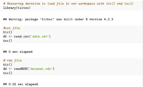
As we can see, tic() and toc() are simple timing functions for basic measurements within an R script, with tic starting the timer before a function to be measured is run and toc to stop the timer.

Benchmarking in R

While on the subject of timing in R, we should also call out and differentiate the difference between timing and benchmarking.

Benchmarking can be used to compare the performance of different implementations. This is different than timing in R as previously described and shown.

Benchmarking in R can be achieved using the benchmark() function from the rbenchmark library package or through the microbenchmark library.

Let’s go through examples of each of these libraries now.

Benchmark Timing in R Example with rbenchmark

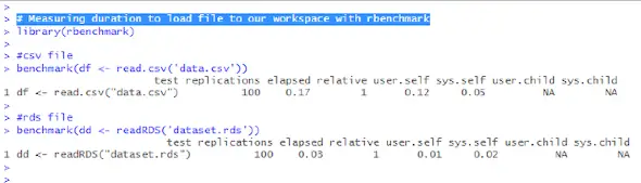
# Measuring duration to load file to our workspace with rbenchmark
library(rbenchmark)

#csv file
benchmark(df <- read.csv('data.csv'))

#rds file
benchmark(dd <- readRDS('dataset.rds'))

The benchmark() function from rbenchmark library can take a list of expressions or functions (just one measured above) and run them multiple times. Measurements of the time taken by each run are determined. Then, it returns a data frame containing the timing results such as the following:

Timing in R with microbenchmark

# Measuring duration to load file to our workspace with microbenchmark()
library(microbenchmark)

# benchmarking, simulating 100 repetitions
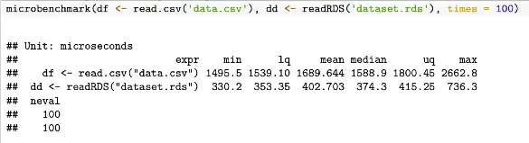
microbenchmark(df <- read.csv('data.csv'), dd <- readRDS('dataset.rds'), times = 100)

With the results from this code example looking like the folllowing

To summarize, benchmarking in R is useful for easily comparing the performance of different implementations as opposed to individually timing portions of R code.

As shown above, rbenchmark and microbenchmark are R packages for benchmarking R code execution time, but they differ in some important ways.

rbenchmark can be useful for benchmarking entire functions or scripts.

On the other hand, microbenchmark provides a more precise and detailed way of measuring the execution time of R code. Compare the two outputs above. microbenchmarking is more often used for measuring the execution time of very small code snippets, such as a single line of code or a small block of code.

Both examples execute the code many times, 100 times by default.

rbenchmark is usually used for timing entire functions or scripts, while microbenchmark is better suited for benchmarking isolated code snippets with higher precision than rbenchmark.

Optimizing Timing in R

By identifying bottlenecks and applying code optimization techniques, R programmers can improve the speed and efficiency of their R code.

Identifying Bottlenecks with Rprof()

One of the first steps in optimizing timing in R is identifying the bottlenecks in the code. Bottlenecks are areas of the code that take up a significant amount of time and slow down the overall execution time of the script.

One way to identify bottlenecks is by using the Rprof() function, which provides a profile of the code and identifies the functions that take up the most time.

If you’d like see a tutorial with Rprof just let me know in the comments below.

R Code Optimization Techniques

Once identified, users can apply R code optimization techniques to address the bottleneck and improve the speed and efficiency of their code.

Some of these techniques include:

Vectorization: vectorized operations, instead of loops, can improve the speed of R scripts.
Caching: Caching frequently used data or results can reduce the amount of time spent recalculating them. Classic trick.

Parallelization: Splitting up tasks and running them in parallel can improve the speed of R scripts especially on multi-core systems.
Memory management: Efficient memory management, such as removing unused objects and avoiding excessive copying, can reduce the execution time of R scripts.

Optimization techniques is a different subject than ways to time code in R, but in short, by applying techniques such as those listed above, R programmers may be able to optimize the timing of their R scripts.

Let me know if interested in more.

R Code Timing External References

Github repo of R Timing Source Code
palmerpenguins data set used throughout the R code timing examples

tidyverse R library used in R glimpse example in setup of examples code above
https://www.alexejgossmann.com/benchmarking_r/
More R Programming Tutorials

Conclusion of R Timing

Timing is an essential aspect of programming in R. In this tutorial, several techniques for measuring R timing were explored.

The tutorial started by describing and providing examples of how to time R code using built-in functions. Next, using R timing library packages was described with code examples shown.

This tutorial then went on to describe differences between timing and benchmarking and again, examples were shown.

Towards the end, optimization techniques, such as vectorization, caching, and parallelization, were mentioned which can significantly speed up R code in some cases.